
What is HPC?
The goal of HPC is to solve very large complex problems as efficiently as possible.
The Work-Span Model
The work-span model assists in understanding the efficiency of an algorithm, especially when parallelized.
Essentially, each algorithm can be represented as a DAG, where each vertex is the operation, and the directed edges shows the operation dependency on one another. Then, with the DAG created for the algorithm, find the work–the number of vertices in the DAG–and the Span–the longest path through the DAG, of an algorithm.
Parallelization
One of the coolest parts of this class was taking many commonly known algorithms, such as BFS, and parallelizing it by having processors assigned to different portions of the task, overall speeding up the process. One example is the List Ranking Problem, which we were assigned to in lab 1 using OpenMP.
Example for-loop in OpenMP:
#pragma omp parallel for
for (int i = 0; i < n; i++) {
   // .. do something here
}
OpenMP automatically splits the tasks of this for loop between the processors (p) of the CPU. Normally, we would have a runtime of a for-loop to be O(n), but with the use of OpenMP, we instead get a runtime of O(n/P), which is faster.
Rather than parallelizing with multiprocessors in the CPU, another alternative parallel computing model that was also used in the assignment is Nvidia’s CUDA, which focuses on parallelization in a GPU, and requires developers to handle the data transfer between the CPU and GPU memory.
Example doFunction in CUDA.
cudaMemcpy(d_x, x, N*sizeof(float), cudaMemcpyHostToDevice);

doFunction<<<1, 256>>>(d_x);

cudaMemcpy(x, d_x, N*sizeof(float), cudaMemcpyDeviceToHost);
Let’s say you had an array x and wanted to manipulate this array in parallel. You would first copy the array to the GPU, perform the function call, specifying the number of blocks and threads to use, 1 and 256 respectively. The function would be performed in the GPU, and lastly, we would transfer the manipulated array from the GPU back to the CPU to use.
Distributed
Now, rather than having processors split up the tasks, we can have tasks divvied up between different computers, necessitating communication between each other. Lab 2 focused on designing efficient communication algorithms for built-in collective algorithms such as MPI’s MPI_Scatter and MPI_Gather.
Example function using MPI.
int function(...) {
   int size, rank;
   MPI_Comm_size(comm, &size);
   MPI_Comm_rank(comm, &rank);
   if (rank == root) {
      MPI_Recv(...); // receive
   } else {
      MPI_Send(...); // send to root
   }
Each computer would run the function, with the size as the total number of processes, and the rank specifying what the rank of the process is (0,1,2,3…). If there were four computers, each would have rank 0,1,2, or 3. Using MPI allowed for algorithm efficiency by divvying up the tasks into subtasks, assigning a process to do the subtask, and combining all the subtasks together.
Alpha Beta Cost Model
To analyze the efficiency of these super computers with distributed memory, since communication is involved, we can assess using the alpha beta cost model, where alpha is the latency to send a message, regardless of the message size, and beta is the inverse bandwidth, which is affected by things such as communication congestion.
T(n) = α + β * n
For example, if there exists congestion of communication of five different nodes trying to communication to one specific node, the beta term would increase 5x, as communication can only be made one at a time.
Class Logistics:
Time Spent: 25hrs/wk
Difficulty: 8/10
Overall Rating: 7/10
Weight distribution:
Lab 0: 10%
Lab 1: 15%
Lab 2: 20%
Lab 3: 20%
Extra Credit Lab: 0%
Midterm: 15%
Final: 20%
Grade: 90.97% (A)
Lab 0: 64/100
Lab 1: 100/100
Lab 2: 96/100
Lab 3: 91.1/100
Midterm Exam: 35/40
Midterm Adjustment: 7/0
Final Exam: 34.5/50
Final Adjustment: 6.5/0
Grade Notes:
Some of the labs were difficult and/or time-extensive.
The midterm and final exams were difficult, with content really testing your knowledge and understanding the lectures. On the bright side, the curves were extremely generous, as we were provided adjustments for both the midterm and final, along with an overall letter grade curve:
82 for an “A”, 69.5 for a “B”, 57 for a “C”
Overall
I think the labs were interesting, but very intensive with not much to go off of. I had to spend a few hours on a lot of the labs to get a basic understanding on what I need to implement. Furthermore, the midterm and finals do not really stem off of your understanding of the labs. I disliked how much time I spent on the labs where barely any of the knowledge was used in the exams. Instead, the exams covered various other topics from the lecture, which, surprise, was not used in a lot of the labs.
Also, many of the TAs were not that helpful in answering questions in the ed post.
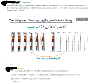
I ended up being able to implement scatter_tree, but could not use scatter_tree to implement broadcast_tree as the steps were very much different, contrary to the TA’s answer of “if you can do scatter_tree, you can do broadcast_tree.” However, there was great collaboration between students which made the class much more manageable.
Despite my dislike for the course structure, I learned a lot, and still found this class worthwhile.